
I created a couple of OSM visualisations for my talk at the OSGeo Ireland conference.
See: History of OpenStreetMap in Ireland
These are pretty easy to make, but take a fair bit of time. I did mine for Ireland, but should work with any part of the world.
Required software:
- PostgreSQL with PostGIS
- Python
- QGIS
- osmium-tools
This is the trickiest part, installing osmium-tools: here.
Data:
An OSM full history export. The best source for these is GEOFABRIK.
For Ireland:
http://download.geofabrik.de/europe/ireland-and-northern-ireland.html
Due to GDPR, you will have to log in with an OSM id to download the full history extracts. User ID’s are personal data.
Process:
The workflow is pretty simple. Osmium-tools provides pretty easy API access to the history files, where you can provide a data, and it will extract what OSM was like at that date. We simply need to loop through the desired dates we want to extract, and pipe the results into a workflow that loads the data into PostgreSQL. The final step is simply rendering in QGIS using the time manager plugin.
Python Script:
Github GIST:
https://gist.github.com/HeikkiVesanto/f01ea54cca499a6a144d18cf8909c940
The tables in the database will be:
- lines
- multilinestrings
- multipolygons
- other_relations
- points
Each feature will be tagged with the date it is associated with.
Visualisation:
To visualise the data in QGIS we use simply use the excellent time manager plugin, filtering on the load_date field and with a monthly interval.
Result:
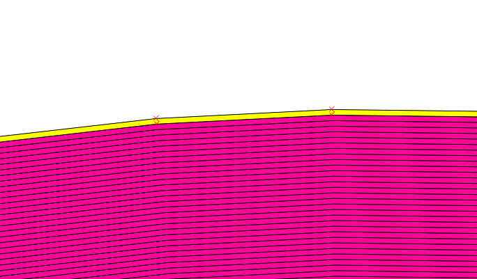
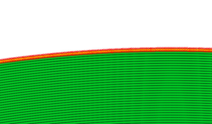
![Screenshot[34]](https://gisforthought.com/media/2015-07-22_19867606025_52077255de_b.jpg)