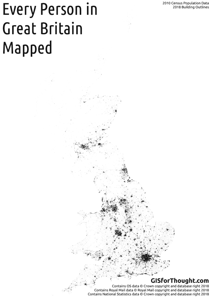
Multi Ring Buffer – Buffer the Buffer or Incrementally Increasing Distance?

Does it matter, and who cares?

Multi-ring buffers can be useful for simple distance calculations as seen in:
X Percent of the Population of Scotland Lives Within Y Miles of Glasgow
And:
X Percent of the Population of Scotland Lives Within Y Miles of Edinburgh

For these I simply created multiple buffers using the QGIS buffer tool. This works for small samples, but was quite frustrating. I had initially hoped to do the whole analysis in SQLite, which worked pretty well initally, but struggled on the larger buffers. It took too long to run the queries, and did not allow for visualisation. I think using PostGIS would however be pretty feasible.

But creating a multi-ring buffer plugin for QGIS also seemed like a good learning experience. Which got me thinking, does it matter if you create increasingly large buffers around the original feature, or if you buffered the resulting buffer sequentially. My hypothesis was that there would be pretty significant differences due to the rounding of corners.

I asked on StackExchange but the conversation did not really take off:
http://gis.stackexchange.com/questions/140413/multi-ring-buffer-methodology

My question is not about the overlapping-ness of the buffers, since I think multi-ring buffers should be “doughnuts” anyway. But rather if smoothing will occur. The only answer was to try it myself.

Buffer styles:
Buffer the resulting buffer sequentially: Sequential
Buffer the original feature with increasing buffer distance: Central
[table caption=”Speed – In seconds”]
Features, Rings,Central, Sequential
1, 5, 0.59, 0.56
55, 5, 8.06, 6.38
1, 200, 60.83, 31.76
3, 200, 62.89, 40.89
55, 200, 628.38, 586.67
1, 2000, 203.84, 67.00
[/table]

No matter how you do it the sequential style is quicker, but that may be down to my code.

Rendering

Interestingly, although understandably, the sequential style results in a lot more vertices in the outer rings. For comparison, for a 500 ring buffer the outermost ring had the following vertice counts:
[table]
Style, Vertices
Central,488
Sequential,30918
[/table]

We can see this with editing turned on.
Central:
Central_editing
Sequential:
Sequential_editing

We can also see a smoother profile in the sequential buffer. However the difference is not major, and hard to discern with the naked eye.

So we have at most about around a 10m discrepancy, with 500 50m rings, so around 25000m of distance from the original feature.
Screenshot[34]
This impacts rendering time dramatically, an example with our 500 rings:

Central:

Sequential:

So quicker to create but slower to draw. So which one is better, quicker calculation, or quicker rendering? Or should we not do 200+ ring buffers?

Hard to say. In version 0.2 of the Multi Ring Buffer Plugin. There is an option for either in the advanced tab.

Plugin: https://plugins.qgis.org/plugins/Multi_Ring_Buffer/
Please report any issues through GitHub: https://github.com/HeikkiVesanto/QGIS_Multi_Ring_Buffer/issues

Mapvember 2014

Mapvember: A map/tutorial a day for every day in November.

Some days had more than one map, some had tutorials, one just had a photo. Some were very easy, others would have take a couple of days of work.

Excellent experience, good learning experience and an opportunity to post previous projects that were a bit short of being great. A little time consuming at times though. I started making the maps around half way through October, so I had almost the first week ready when November began, but the days ticked by quickly. Happy to have done it. I encourage everyone to join in next year, or any other month.

Visitor Statistics:

Total views: 3047
Uniques: 2289
Pageviews: 4327

Top 10 Countries:
United Kingdom: 1147
United States: 363
Germany: 183
France: 120
Canada: 85
Italy: 67
Spain: 66
Australia: 56
Switzerland: 42
India: 39

Mapvember Countries

Top 10 Cities:

Glasgow: 340
London: 212
Edinburgh: 122
Rostock: 45
Aberdeen: 42
Stirling: 35
San Jose: 31
Vienna: 28
Berlin: 28
Zagreb: 26

Mapvember Cities

Other Months:
August Visitors: 303
September Visitors: 641
October Visitors: 523
November Visitors: 3047

Most popular posts:
X Percent of the Population of Scotland Lives Within Y Miles of Glasgow – 521
Glasgow Subcrawl Map – 400
Polygon Outlines in QGIS – 276
Setting up PostgreSQL and PostGIS on Linux Mint (Not posted in November) – 258
Glasgow 3D Residential Property Density QGIS2threejs – 218
Georeferencing Vector Data Using QGIS and ogr2ogr (Not posted in November) – 173
Great Circle Flight Lines in Postgis – 171
London Bus Route Maps – 154
Centroid Within Selection in QGIS – 114
QGIS Inverse Shapeburst Fills – 109

Referrals:

Reddit.com: 747
OSGeo.org: 381
Twitter: 122
GIS.StackExchange.com: 71
Facebook: 70
Flickr: 15

Top SubReddits:

/r/glasgow: 200
/r/scotland: 120
/r/london: 46
/r/gis: 19
/r/QGIS: 4

Thanks for visiting.

Great Circle Flight Lines in PostGIS

There is an excellent post by Anita Graser about creating Great Circles in PostGIS.

However as of PostGIS version 2.1 this can be done in a different (better) way, using the geography functions.

PostGIS Great Circles

For more information about geography, see:
Introduction to PostGIS – Geography

This allows us to create the great circles without having to add in a new projection.

So we first need to create our three tables in PostGIS:

CREATE TABLE airlines

(Airline_ID integer,Name varchar,Alias varchar,IATA varchar,ICAO varchar,Callsign varchar,Country varchar,Active varchar, uid Serial);
CREATE TABLE routes

(Airline varchar,Airline_ID integer,Source_airport varchar,Source_airport_ID integer,Destination_airport varchar,Destination_airport_ID integer,Codeshare varchar,Stops varchar,Equipment varchar, uid Serial);
CREATE TABLE airports

(Airport_ID integer,Name varchar,City varchar,Country varchar,IATA varchar,ICAO varchar,Latitude double precision,Longitude double precision,Altitude double precision,Timezone double precision, dst varchar, tz varchar, uid Serial);

The data itself can be found at: openflights.org/data.html

We can then load our data through PGAdminIII. You can just right click on a table and select import. Remember to not load the “uid” column, because it is our primary key which will be populated automatically and not in the original data. You will also want to define it as the primary key.

Now we need a geometry column in the airports dataset.

ALTER TABLE airports ADD COLUMN geom geometry(POINT,4326);

We can define our geometry in the airports dataset from the Latitude and Longitude columns.

UPDATE airports SET geom = ST_SetSRID(ST_MakePoint(longitude,latitude),4326);

And create a spatial index.

CREATE INDEX idx_airports_geom ON airports USING GIST(geom);

Then we can create a flights table.

CREATE TABLE flights AS

SELECT

  air1.geom AS source_geom, 

  air2.geom AS destination_geom, 

  airlines.name, 

  routes.equipment, 

  routes.destination_airport_id, 

  routes.source_airport_id, 

  routes.destination_airport, 

  routes.source_airport

FROM 

  public.routes, 

  public.airlines, 

  public.airports air1, 

  public.airports air2 

WHERE 

  routes.airline_id = airlines.airline_id AND

  routes.source_airport_id = air1.airport_id AND

  routes.destination_airport_id = air2.airport_id;

This table will have a source geometry and a destination geometry along with a few other attributes. I added a primary key to this table as well.

To filter out a specific airport, for example Honolulu we use the “Airport ID”.

CREATE TABLE honolulu_flights AS

SELECT * FROM flights

WHERE destination_airport_id = 3728 OR source_airport_id = 3728;

Then we add in the actual line geometry column.

ALTER TABLE honolulu_flights ADD COLUMN line_geom geometry(LineString,4326);

And populating the great circle geomtrey:

UPDATE honolulu_flights

SET line_geom =  

  (ST_Segmentize(

  (ST_MakeLine(source_geom, destination_geom)::geography)

  ,100000)::geometry)

;

This is works great to an extent, but QGIS still has some trouble with lines that cross the date-line.

Screenshot[32]

We can fix this using a Pacific centered projection like EPSG:3832.

Screenshot[33]

We can either set QGIS to the projection. Or we can set our geometry to this projection when creating the flight lines.

ALTER TABLE honolulu_flights ADD COLUMN line_geom geometry(LineString,3832);
UPDATE honolulu_flights

SET line_geom =  

  ST_Transform((ST_Segmentize(

  (ST_MakeLine(source_geom, destination_geom)::geography)

  ,100000)::geometry), 3832)

;

Thanks to:
The World Is A Village – PostGIS: using latitude and longitude to create geometry
http://gis.stackexchange.com/questions/84443/what-is-this-postgis-query-doing-to-show-great-circle-connections

Population of Scotland Mapped

An updated version can be found at: Every Person in Scotland on the Map

One random point on the map for each person within a postcode in Scotland.

Workflow:
OS Code-Point Open points.
>
Voronoi polygons from the postcodes.
>
Join 2011 Scottish Census postcode population counts to Voronoi polygons.
>
Clip the resulting polygons to the Scottish coastline (using PostGIS for time saving).
>
Intersect the lakes out of the resulting polygons.
>
Random point in polygon into the postcode Voronoi polygons (minus lakes), using the census counts.
>
Output:

Population of Scotland Mapped

An easier approach would have been to use the NRS supplied postcode areas for Scotland mentioned in previous posts. A better display of this data would be through a web mapping environment, which is working on my home environment but lacking hosting.

Centroid Within Selection in QGIS

Edit – This can now be done using a plugin: QGIS Select Within Plugin

While we have some options for spatial selection in QGIS through the Spatial Query plugin. One option that is glaringly missing is centroid within. This is extremely useful for easily selecting polygons that mainly fall within other polygons. This tutorial will run through how to do a polygon centroid within another polygon selection in QGIS.

Our initial setup is a postcode dataset, where we want to extract all of the ones that are mainly within Glasgow City Council. The boundaries are not the same but are roughly the same. However an intersect query would bring ones that simply touched the area, and a within query would exclude the ones that fall just outside. A centroid within should work great.

Selection

In this image the red lines are our postcodes, and the yellow area is the highlighted Glasgow City polygon.

We are going to cheat slightly by using SpatiaLite, which is a stand alone, single file, spatial database. It is however very tightly integrated into QGIS and we do not have to leave the program so I feel this counts as a QGIS solution.

First using one of the browser panels create a new database:

Screenshot[34]

Transfer your data into the database. This can be done by dragging and dropping a .shp file into the newly created database using two browser panels.

I created a subset of the postcode dataset, with a simple polygon selection of roughly the Glasgow area (postcode_glasgow_nrs_rough). My other dataset is the UK unitary authorities dataset (district_borough_unitary_region).

Then open up the DB Manager. Database>DB Manager>DB Manager.

Once in the database we can do the query using simple SQL:

SELECT  postcode_glasgow_nrs_rough.*

FROM postcode_glasgow_nrs_rough

JOIN district_borough_unitary_region

ON ST_intersects(ST_centroid(postcode_glasgow_nrs_rough.geom),district_borough_unitary_region.geom)

WHERE district_borough_unitary_region.name LIKE "%lasgow%"

We also have a WHERE statement so only the ones that within Glasgow are selected. “%lasgow%” used to avoid capitalization mismatches.

Screenshot[35]

We can also directly add this query in as a layer in QGIS using the “Load as new layer” feature. An excellent feature, and only requires you to select the primary key and geometry column. This allows us to visually check our results.

The query has worked as intended, but we have some strangely shaped polygons so the results are not what I had hoped.

Screenshot[37]

We can see that one of the postcode polygons is missing from the selection because its centroid actually falls outside of itself.

Not to worry we have a better option than centroid for this query, which is ST_PointOnSurface. Details can be found on the Boundless PostGIS pages.

So lets try this.

SELECT  postcode_glasgow_nrs_rough.*

FROM postcode_glasgow_nrs_rough

JOIN district_borough_unitary_region

ON ST_intersects(ST_PointOnSurface(postcode_glasgow_nrs_rough.geom),district_borough_unitary_region.geom)

WHERE district_borough_unitary_region.name LIKE "%lasgow%"

Screenshot[36]

Adding it in we see the results as expected.

Screenshot[38]

So great we now have our data selected, but how do I get it out of SpatiaLite? We could wait for the “Load as new layer” to load in all the features, then save it as a shapefile, but for my query, while great for quick look, the “Load as new layer” was running quite slow and thus not an option.

So instead, we can simply create a new table in the database from our selection.

CREATE TABLE glasgow_postcode_nrs AS

SELECT  postcode_glasgow_nrs_rough.*

FROM postcode_glasgow_nrs_rough

JOIN district_borough_unitary_region

ON ST_intersects(ST_PointOnSurface(postcode_glasgow_nrs_rough.geom),district_borough_unitary_region.geom)

WHERE district_borough_unitary_region.name LIKE "%lasgow%";

Note the ; at the end. This creates a new table pretty quickly. And to get it to appear as a spatial table we simply register its geometry in the geometry column:

INSERT INTO geometry_columns VALUES ('glasgow_postcode_nrs', 'geom',6, 2, 27700, 0);

With the options being: Table name, Geometry column, Geometry (type 6 for polygon), dimensions, SRID, Spatial index boolean.

The table the appears in our browser.

Screenshot[41]

And our final result.

part2

I am loving the database integration in QGIS. It makes some workflows much easier and adds a wealth of new opportunities. Also the “Load as new layer” views are amazing, lots of possibilities.